'Can we Descend Deeper' : Some Optimization Techniques in Machine Learning
I'm currently halfway through my MA630 course (Optimization Methods) at Stevens, and it's been a blast.
I've learned about a lot of things.
Initially, I was thinking of writing a blog series about the content from this class.
However, I'd like to start off by combining some of the concepts I've learned so far with
my previous knowledge - machine learning.
NOTE: This blog assumes that you have a background in vector calculus and linear algebra. You don't necessarily have to know
too much about machine learning to follow along, but some familiarity would help!
Background: Machine Learning
I will define machine learning as the process of training a model to make predictions based on data. The model itself
can be a bunch of different things - anything from a linear regression model (, predicts a continuous value)
to a neural network is valid.
All models have parameters. These are the "knobs" that we can turn to change how the model behaves. For example,
a linear regression model has two parameters: m (slope) and b (y-intercept). Meanwhile, something like a neural network would have
many more parameters.
The process of training a model involves finding the best parameters (weights) for the model such that it minimizes
some "loss function" - a function that measures error between the model's predictions and the actual values.
As an example, let's say we have a model that predicts whether or not an email is spam. This model can be ANYTHING.
The important part is the output: a prediction of spam or not spam.
To convert this prediction into a number, let's say we use 1 for spam and 0 for not spam.
For something like this, we will use a loss function called "binary cross-entropy loss".
Given the "true label" y (1 for spam, 0 for not spam) and the predicted probability (between 0 and 1),
This function will increase as the predicted probability goes further away from the true label. From here, we want to find a way to make this as small as possible.
More Background: Convexity and its Importance
A good chunk of loss functions have nice mathematical properties: convexity and differentiability.
If you've taken a calculus class before, you probably know what convexity is.
A function is convex if, for any two points on the function, the line segment connecting those two points lies above
the function itself (also known as an epigraph).
This can also be defined in mathematical terms.
This property is super important in optimization because it guarantees that any local minimum value of a convex function is
also a global minimum value. This means that if we find a point where the function's slope is zero (a local minimum),
we can be sure that this point is the absolute lowest point on the function.
Because of this, convex functions are much easier to optimize. We know a lot more about their behavior, and we can use techniques like gradient descent!
What is Gradient Descent?
I'm sure that you've learned about critical points before to find minima and maxima of functions. You take the derivative of the function,
set it to zero and solve for the variable. Why don't we just do that?
Well, this method works for simple functions with one or two parameters. But what about functions with hundreds? Thousands?
Extending our linear regression example, let's generalize our formula:
Y can be a vector of outputs, X is a matrix of input features, is a vector of parameters (weights), and is the intercept (bias).
What happens when is a 10,000-dimensional vector? We'd have to take the derivative of the loss function with respect to each of those 10,000 parameters,
set them to zero, and solve a system of 10,000 equations!
These kinds of operations are extremely expensive to compute. We need a more efficient way to find a minimum.
Enter, gradient descent! Gradient Descent (which I will notate as GD) is an iterative optimization algorithm to find minima.
Instead of finding a closed form solution (directly solving the system of equations), GD takes small steps in the direction of the steepest descent to find a minimum.
(As a note, the steepest descent is given by the negative of the gradient of the function at a given point.)
Going back to why convexity is important - it gives us a function that's almost like a bowl. If we start at any point on the bowl,
we can follow the steepest descent to reach the bottom of the bowl (the global minimum).
Here's what the update rule for Gradient Descent looks like!
- Initialize parameters (in this case, ) randomly
- Compute the gradient of the loss function with respect to the parameters.
- Update the parameters by taking a step in the direction of the negative gradient.
- Repeat steps 2 and 3!
The update rule can be summarized mathematically as:
where β represents the parameters, α is the learning rate (step size), and ∇L(β) is the gradient of the loss function with respect to the parameters.
The learning rate controls how much of a "step" we take in the direction of the negative gradient!
There are different ways to choose the learning rate! They can generally be classified into two categories:
- Fixed learning rate: A constant value throughout the training process.
- Adaptive learning rate: Adjusts the learning rate based on the progress of the optimization
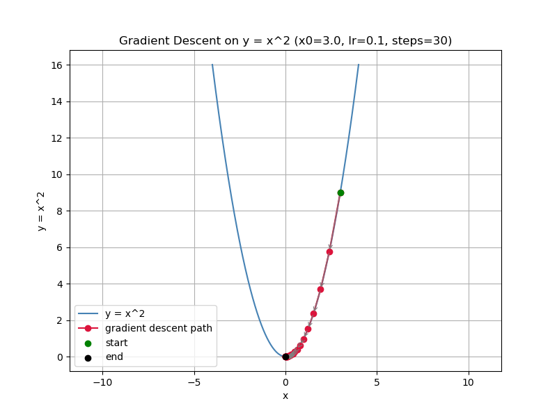
A simulation of gradient descent on a simple 2D parabola
As a note, GD does work with functions that are not convex. However, we may end up in local minima instead of global minima.
So, here's the question: how fast does GD usually converge?
Understanding Speed of Convergence
Here's where I have to start citing my sources. There's a lot of proofs from here on.
One important part that we'll cover is the speed of convergence (how fast we reach the minimum).
We will use this to compare GD to other optimization techniques later on!
Let's update GD's rule to make it a sequence. Let's let be our parameters at "iteration" . Then, for any objective function ,
Same idea, but now we want to analyze how fast converges - as a sequence - to the optimal solution .
Now, we need some definitions for a mathematical analysis.
Def: Lipschitz Continuity
A function is said to be Lipschitz continuous (or L-smooth) with constant if, for all ,
In simpler terms, this means that the rate of change in the function can be bounded by a constant .
Def: Strong Convexity
A function is strongly convex with parameter if, for all and ,
Kind of the opposite of Lipschitz continuity - this means that the function has a lower bound on its curvature. You can kind of see the similarity between this and a normal convex function's definition!
Th: GD Convergence Rate (L-Smooth Functions) [1]
The speed of convergence of GD depends on the properties of the function that we are trying to minimize.
If is convex and its gradient is Lipschitz continuous with constant ,
then the following property holds for with a fixed learning rate :
If we disregard (where we start), we can see that the error generally decreases at a rate of . This is known as a sublinear convergence rate - the convergence slows down as we get closer to the minimum. Pretty slow.
Th: GD Convergence Rate (Strongly Convex Functions) [1]
If is strongly convex with parameter and its gradient is Lipschitz continuous with constant , then the following property holds for GD with a fixed learning rate :
The error now decreases at a rate of , which is known as a linear convergence rate. In other words, the error decreases at a constant rate. This is better!
What if the function is not convex at all?
If the function is not convex, GD may still converge, but there are no guarantees on the convergence rate.
As we can see, the properties of the function are important in determining how fast an optimization algorithm converges.
Now, we can explore other optimization techniques and compare their convergence rates to GD!
Newton's Method
Newton's Method is another optimization algorithm, but it uses second-order information (the Hessian matrix) to find the minimum while
GD only uses the first-order information (the gradient).
The update rule for Newton's Method is given by:
where is the Hessian matrix of second derivatives at point .
That being said, calculating the inverse of the Hessian can be computationally expensive. In practical cases, the Hessian is
factorized to avoid direct inversion [3]. A common example of this is the Cholesky decomposition.
Using the Hessian lets Newton's Method take advantage of the curvature (possibly convexity) of the function to make better updates.
This is especially useful for functions that are strongly convex (and ESPECIALLY quadratic functions).
To demonstrate this, let's look at this problem:
Well, to simplify things from matrices/vectors to scalars, let's say:
This is a simple 3D quadratic function. The gradient and Hessian are:
Here, we know that the minimum is at (0, 0). This can be calculated by hand.
If we were to simulate GD and Newton's Method on this function from the point , we would see something like this (looking at the 2D contour plot):

Gradient Descent (with optimal learning rate)
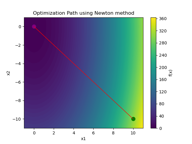
Newton's Method
Gradient Descent took 16 iterations to converge, while Newton's Method took 1 iteration! That's a huge difference! However, as we will see later, Newton's Method may be inefficient in other situations.
Th: Speed of Convergence of Newton's Method (PD Hessian) [2][3]
(NOTE: This theorem assumes that we use the two-slope test for step size selection. I never covered this, but just assume we can find a reasonably optimal step size per iteration.)
If our function is twice continuously differentiable and the Hessian is positive definite for all
in the bounded set ,
then the following statement is true:
This tells us that Newton's Method will converge to the optimal solution at a superlinear rate. It's
faster than linear convergence, meaning that the error decreases more rapidly as we get closer to the minimum.
On top of this, if the Hessian is Lipschitz continuous within , then we can get an even stronger convergence rate:
is the Lipschitz constant of the Hessian, and is the smallest eigenvalue of the Hessian within .
This means that the error decreases quadratically as we get closer to the minimum!
Why don't we always use Newton's Method?
Newton's Method is great when it comes to looking at convergence rates for convex functions. However, there are some downsides.
The biggest one is computational cost. Calculating the Hessian (not to even mention its inverse) is extremely expensive for high-dimensional problems.
Even with factorization methods, the time complexity is still for an -dimensional problem.
Thus, let's try to estimate the Hessian instead of calculating it directly.
Quasi-Newton Methods
Quasi-Newton Methods are a class of optimization algorithms that aim to approximate the Hessian matrix instead of calculating it directly. This reduces the computational cost while still taking advantage of second-order information.
There are two methods that I want to go over: the nonlinear Conjugate Gradient (CG) method and the Limited-memory Broyden-Fletcher-Goldfarb-Shanno (L-BFGS) method.
Def: Conjugate Gradient Method
The Conjugate Gradient (CG) method is - like the original gradient descent - iterative. It is based on solving a set of linear equations, but it is adapted for nonlinear optimization problems.
To be continued... (This blog was originally made in November 2025, and I wanted to release it ASAP, but I am still working on it. Thus, I will release it now and continuously work on it.)
References:
[1] Garrigos, G., & Gower, R. M. (2024). Handbook of convergence theorems for (stochastic) gradient methods (arXiv Preprint arXiv:2301.11235). arxiv.org/abs/2301.11235
[2] Martínez, J. M., & Qi, L. (1995). Inexact Newton methods for solving nonsmooth equations. Journal of Computational and Applied Mathematics, 60(1-2), 127–145. doi.org/10.1016/0377-0427(94)00088-I.
[3] Ruszczynski, A. (2011). Nonlinear optimization. Princeton University Press. ISBN-13:978-0691119151, ISBN-10: 0691119155