Disclaimer: While this project was created for fun, it is not intended to replace the human creativity and skill that goes into creating high-quality beatmaps. This project is purely an exploration of what is possible with machine learning and deep learning, and it is not intended to be used for any serious purposes.
I recently had the honor of graduating with my Master's Degree in Data Science, and I'm currently waiting to start working. In my free time, I've spent most of my time - honestly - bumming around. However, I wanted to make sure that my technical chops were still there.
Part of my bumming routing includes playing "osu!" - a rhythm game where you click circles in time with music. I've played it for a few years, and I'm currently trying to hit a 5 digit global rank. You can actually find my osu profile here. I realized that there was potential to use the skills I learned to make something interesting - a tool that could generate beatmaps.
Small Note :3
I will try to explain some concepts at a higher level, but this blog will be more enjoyable to read if you have some prior knowledge of machine learning and deep learning. It will also be more enjoyable if you have a fundamental understanding of how osu is played (as long as you've seen/played the game, that's more than enough). The full topic list is provided below.Osu Topics:
Machine Learning Topics:
The Idea & Original Thinking (June 2024)
This idea was formulated and briefly worked on about two years ago. I recruited one of my friends, and we developed a basic idea.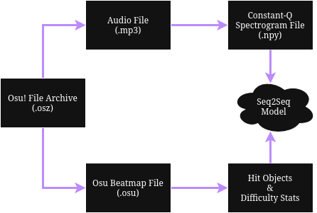
A basic model idea using Seq2Seq
The maps that users download are made by other people, and they are downloaded as an .osz file. However, we found out through some research (two google searches) that .osz files are just ZIP files. Extracting from an .osz file reveals the contents of each beatmap in the form of an .osu file, along with any other assets (images, audio files, etc.) used in the beatmap.
From here, we can take the beatmap's audio file and turn it into structured data - a spectrogram. Our original spectrogram was a constant-Q spectrogram, and we didn't think about the specific type of spectrogram that much. We went with default settings - 84 bins, spanning 7 octaves of notes (logarithmic scaling of frequencies to adjust to human perception).
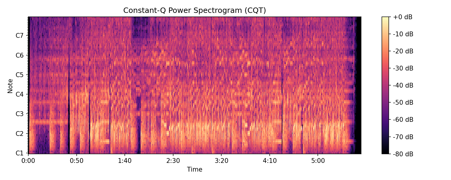
An example of a Constant-Q spectrogram
Since spectrograms can be represented as 2D matrices, we saved all the spectrograms as .pkl files (this was before the picklescan vulnerabilities were found).
From there, supervised learning would be used. We built an Seq2Seq (Encoder/Decoder) model to take in the spectrogram and predict hit objects. The encoder was tasked with embedding the spectrogram into a contextualized "hidden state" through a bidirectional LSTM, while the decoder used the hidden state to predict the next hit object with a 2-layer unidirectional LSTM. The reason the decoder had to be unidirectional was because it was using teacher forcing (we fed the previous actual hit object into the decoder to predict the next hit object).
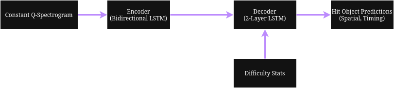
Our original Seq2Seq model idea
The more specific aspects of the model (i.e. the layer shapes) can be found in the table below.
Detailed Tensor Shape Directory
B = 1 (number of songs trained at a time), T = Number of Spectrogram Time Steps
| Layer / Stage | Variable | Shape |
|---|---|---|
| Input Audio | $y$ | $(N_{\text{samples}},)$ |
| Acoustic Transform | $S$ | $(84, T)$ |
| Encoder Input | $x$ | $(B, T, 84)$ |
| Encoder Output Sequence | $\text{encoder\_out}$ | $(B, T, 128)$ |
| Encoder Recurrent State | $\text{encoder\_hc}$ | $(2, B, 64)$ |
| Decoder Input (Step) | $\text{decoder\_input}$ | $(B, 1, 14)$ |
| Decoder Recurrent State | $\text{decoder\_hidden}$ | $(2, B, 64)$ |
| Decoder LSTM Output | $x$ (in $\text{forward\_step}$) | $(B, 1, 64)$ |
| Decoder Hidden Layer | $\text{hidden}$ | $(B, 1, 32)$ |
| Decoder Output Layer | $\text{out}$ (in $\text{forward\_step}$) | $(B, 1, 8)$ |
| Accumulated Output | $\text{decoder\_outputs}$ | $(T_{\text{target}}, 8)$ |
The numbers in most of these layers were arbitrarily picked, but let's go over the important numbers.
The input audio has $N_{samples}$ samples - the number of audio samples in a given audio file. Each spectrogram is "sliced" at certain intervals (in this case, 46ms), and each slice is passed through the encoder sequentially. For a song that's about 3 minutes, there's about 4000 time steps.
From there, we pass it through a bidirectional LSTM to embed the spectrogram. This is done in the hope that the model will capture the "essence" of the song and compress it into some more efficient representation. The reason the LSTM is bidirectional is because we want to capture both past and future information for the sake of continuity in rhythm.
The decoder is now tasked with taking this representation and producing hit objects. The accumulated output layer has a size of $(T_{\text{target}}, 8)$, where $T_{\text{target}} = (N_{\text{samples}})$ and 8 represents the following variables:
While this model seemed okay in theory, it struggled to produce beatmaps because of the way that we encoded our desired output. To process an osu beatmap, we couldn't just put the .osu file into our program since each file had multiple parts such as metadata, difficulty settings and hit objects. Because of this, we embedded all the hitobjects into a 2D array based on their time values.
Every millisecond, we would check if a hit object existed. If so, we would mark its properties. Otherwise, we would fill the columns with 0s. An example is provided below.
| Time Step | x | y | time | type | curveType | slides | length | endTime | Description |
|---|---|---|---|---|---|---|---|---|---|
| ... | 0 | 0 | 0 | 0 | 0 | 0 | 0 | 0 | Silence / Empty space |
| 999 ms | 0 | 0 | 0 | 0 | 0 | 0 | 0 | 0 | Silence / Empty space |
| 1000 ms | 256 | 192 | 1 | 1 | 1 | 0 | 0 | 0 | Hit Circle |
| 1001 ms | 0 | 0 | 0 | 0 | 0 | 0 | 0 | 0 | Empty space |
| 1002 ms | 0 | 0 | 0 | 0 | 0 | 0 | 0 | 0 | Empty space |
| 1003 ms | 100 | 100 | 1 | 2 | 1 | 1 | 120.0 | 0 | Slider |
| 1004 ms | 0 | 0 | 0 | 0 | 0 | 0 | 0 | 0 | Empty space |
| 1005 ms | 0 | 0 | 0 | 0 | 0 | 0 | 0 | 0 | Empty space |
| 1006 ms | 256 | 192 | 1 | 8 | 1 | 0 | 0 | 3000 | Spinner |
| 1007 ms | 0 | 0 | 0 | 0 | 0 | 0 | 0 | 0 | Empty space |
| ... | 0 | 0 | 0 | 0 | 0 | 0 | 0 | 0 | Empty space |
Most of the time steps are - naturally - empty. Because of this, our Seq2Seq model struggled to converge at anything meaningful, as it would always predict a 'no object' time step, leading to a loss of 0 (or whatever our baseline loss was) over time. This was simply not an effective way to represent the problem. We needed something more efficient.
Unfortunately, life got in the way, and we had to stop working on this project for a bit.
The Present: Decentralization
Ok, back to the present and bumming around.Looking at this problem again, I wanted to take a different approach. I hypothesized that one of the other reasons for the failure of the original model was its monolithic nature. The process of both rhythm detection and spatial placement was done in one model, and I realized that we could decouple this into two separate models.